Since the early days, people are faced with making decisions based on choices at the…
Regression Analysis or Trend Estimation
Regression analysis or trend estimation of a series of data points, e.g. observed as a time series, can be regarded as a process of constructing a curve that has the best fit to those data points.
Curve can be used as an aid for data visualization. Time series analysis can reveal unexpected trends in current data, and predict or forecast future trends. As such, it is used across many disciplines and industries.

BusinessQ uses regression method of least squares for calculating a curve or mathematical function. By using calculated mathematical function, BusinessQ visualizes new data points (y-axis or ordinate) that will show the trend estimation of the observed business measure, for example in time.
Types of regression that can be used are:
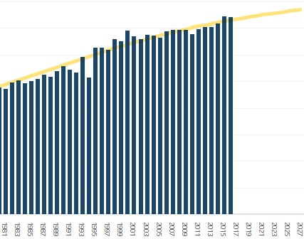
- Linear trend usually shows whether something increases or decreases at a steady rate. We can say that Linear Regression is the most widely used machine learning algorithm for predictive analysis.
- Logarithmic trend is most useful when the rate of change in the data increases or decreases quickly.
- Polynomial trendline is a curved line and it is useful e.g. when you have to analyze gains and losses over big data set. Order of polynomial can be determined by the number of fluctuations in the data.
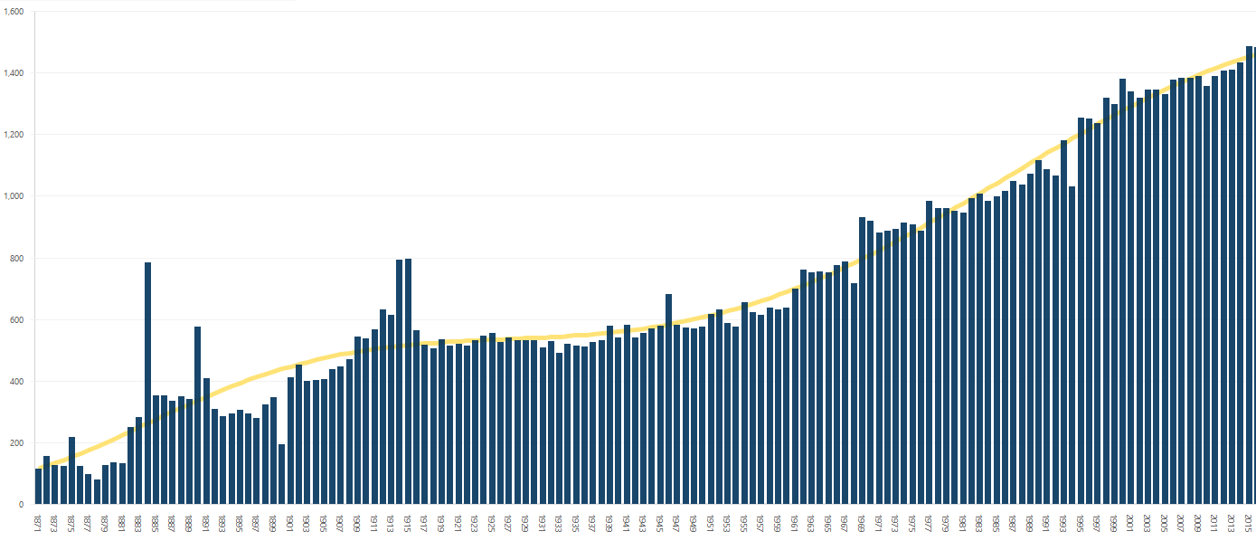
Besides visualizing trend estimation, BusinessQ also shows the exact mathematical function and coefficient of determination, denoted as R2 (“R squared”).
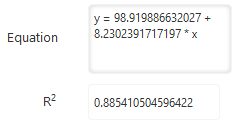
Coefficient of determination represents the fraction of the total variation in the values of y (observed business measure) that is explained by relationship between x (e.g. time) and y (observed business measure). Its value is between 0 and 1. When it is close to 1, trend estimation fits data well. For example, by using linear regression on only two data points, R2 would be 1 because a trendline would perfectly fit two data points; the same would be true for three points and 2nd degree polynomial, four points and 3rd degree polynomial, etc. When there are more points than the degree of polynomial, value of R2 will most likely be lower than 1. In our example R2 is 0.885410504596422, which means approximately 88.54% of the variation in business measure can be explained by the calculated least squares regression.
BusinessQ also has a forecast (extrapolation) feature which allows you to select a number of additional data points that can, for example, show you future trends.
High-order polynomial extrapolation must be used with due care because they may yield unusable values – error of the extrapolated value may grow with the degree of polynomial extrapolation.
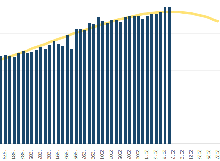
This is related to Runge’s phenomenon – problem of oscillation at the edges of an interval that occurs when using polynomial interpolation with polynomials of high degree over a set of equispaced interpolation points.
I hope BusinessQ regression models will help you see hidden patterns in your data or to spot business trends on time!
Bibliography:
- Regression analysis. (2018, January 19). In Wikipedia, The Free Encyclopedia. Retrieved from https://en.wikipedia.org/w/index.php?title=Regression_analysis&oldid=821311103
- Chapter 3 Examining Relationships. The Practice of Statistics SE (2003): Yates, Moore, Starnes. Retrieved from http://www.henry.k12.ga.us/ugh/apstat/chapternotes/sec3.3.html
- Curve fitting. (2018, January 19). In Wikipedia, The Free Encyclopedia. Retrieved from https://en.wikipedia.org/w/index.php?title=Curve_fitting&oldid=821310968
- (2018, January 17). In Wikipedia, The Free Encyclopedia. Retrieved from https://en.wikipedia.org/w/index.php?title=Extrapolation&oldid=820973168
- Runge’s phenomenon. (2017, December 30). In Wikipedia, The Free Encyclopedia. Retrieved from https://en.wikipedia.org/w/index.php?title=Runge%27s_phenomenon&oldid=817692097
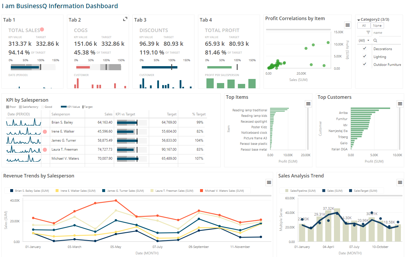
We are developers of data visualization software BusinessQ. Try it for free and make reports and dashboards that make sense, without chart junk.
Related posts